When Does a City Shine Brightest?

When Does a City Shine Brightest?#

Nighttime lights over Seville and the Andalusian coast

Every other tutorial in this book measures sunlight bouncing off the Earth. This one measures light the Earth emits on its own, at night, which is almost entirely a measure of people: streets, ports, greenhouses, industry, and the nights a city decides to celebrate something.

The question here is not how much light there is — that map is well known and boring, the cities are bright and the countryside is dark — but when. Which night of the year does each pixel of a city reach its maximum? get_peak_period() answers that for any index and any dataset, and nighttime lights are where the answer can be checked against something we already know: Seville’s Feria has a date.

The notebook does two things:

The night of the peak, with the daily product over Seville in 2017 — and a hard look at how much of that map is signal and how much is moonlight, clouds and luck.
Forty years of coastal growth, joining DMSP-OLS (1992-2013) to VIIRS (2014-) along the Andalusian coast, and being honest about what can and cannot be compared across that seam.

The method of the first part is the one in Ramírez et al. (2023), which mapped the month of peak radiance for every urban pixel on Earth and found that it moves with the calendar of each country’s festivities.

1. Setup#

import warnings
warnings.filterwarnings('ignore', category=UserWarning, module='geemap.conversion')

import datetime as dt

import ee
import numpy as np
import pandas as pd
import matplotlib.pyplot as plt
from matplotlib.colors import ListedColormap
from urllib.request import urlopen
from PIL import Image
from io import BytesIO

from ndvi2gif import NdviSeasonality

# ee.Authenticate()          # only the first time
ee.Initialize(project='your-project-id')
print('✓ Earth Engine initialised')

✓ Earth Engine initialised

*** Earth Engine *** Share your feedback by taking our Annual Developer Satisfaction Survey: https://google.qualtrics.com/jfe/form/SV_9oS0DRcPvElRMNw?source=python

2. Three datasets, one signal#

ndvi2gif exposes the night in three flavours, and the choice decides what questions can be asked:

`sat=`	Collection	Cadence	Span	Resolution
`'VIIRS'`	`NOAA/VIIRS/DNB/MONTHLY_V1/VCMSLCFG`	monthly	2014-	~500 m
`'VIIRS_DAILY'`	`NASA/VIIRS/002/VNP46A2`	daily	2012-	~500 m
`'DMSP'`	`NOAA/DMSP-OLS/NIGHTTIME_LIGHTS`	annual	1992-2013	~1 km

The daily one is the Black Marble product, and the difference is not only cadence: it models away moonlight, atmospheric scattering, terrain and viewing angle, so one night can be compared with the next. That is what makes a date of maximum meaningful instead of merely arithmetic. With cloud_filter=True (the default) ndvi2gif also applies the product’s own quality flag, keeping the retrievals graded as good and dropping the rest.

The monthly product is what the paper used, and it is cheaper: one image per month instead of thirty.

# Central Seville: the historic centre, the river and the Feria grounds
SEVILLE = ee.Geometry.Rectangle([-6.02, 37.35, -5.93, 37.42])

daily = NdviSeasonality(roi=SEVILLE, sat='VIIRS_DAILY', index='ntl', key='mean',
                        periods=365, start_year=2017, end_year=2017)

print('periods:', daily.periods)
print('first period:', daily._period_date_range(2017, 0))
print('last period: ', daily._period_date_range(2017, 364))

There we go again...
VIIRS Black Marble daily nighttime lights (2012-present, ~500m resolution)
Applying pixel-level quality mask using Mandatory_Quality_Flag
periods: 365
first period: ('2017-01-01', '2017-01-02')
last period:  ('2017-12-31', '2018-01-01')

periods=365 splits the year into single days. Any number works — 4 seasons, 12 months, 24 fortnights, 73 pentads — and get_peak_period() returns the index of the period that holds the maximum, so the unit of the answer is whatever the periods are.

3. The night of the peak#

get_peak_period() builds one candidate per period and lets qualityMosaic pick the winner, so periods with no valid retrieval simply do not compete. Three arguments matter here:

mask_below= drops pixels whose peak never reaches a threshold. The date of maximum of an unlit field is the date its noise happened to be highest, which is nothing at all.
return_peak_value=True keeps the radiance at the peak, to judge whether the maximum stands out or is one of many similar nights.
return_ties=True counts how many periods reach that same maximum. The library does not invent a winner when several tie — it says so, and lets you decide.

peak = daily.get_peak_period(mask_below=5, return_peak_value=True, return_ties=True)
peak.bandNames().getInfo()

Year 2017: 365/365 periods with data using ntl index

['peak_period', 'peak_value', 'ties']

def peak_dates(image, roi, year=2017, scale=500, top=12):
    """Most frequent peak days inside an ROI, as real dates."""
    # eq() at the native scale: a frequency histogram of a composite without a
    # fixed projection invents fractional counts for values no pixel holds
    doys = image.select('peak_period').reduceRegion(
        ee.Reducer.frequencyHistogram(), roi, scale, maxPixels=1e9
    ).getInfo()['peak_period']
    rows = [(int(float(d)), n) for d, n in doys.items()]
    rows.sort(key=lambda r: -r[1])
    jan1 = dt.date(year, 1, 1)
    return pd.DataFrame(
        [{'day of year': d,
          'date': jan1 + dt.timedelta(days=d - 1),
          'pixels': round(n)} for d, n in rows[:top]]
    ).set_index('day of year')

peak_dates(peak, SEVILLE)

	date	pixels
day of year
81	2017-03-22	38
123	2017-05-03	15
139	2017-05-19	13
341	2017-12-07	12
150	2017-05-30	9
96	2017-04-06	9
126	2017-05-06	8
129	2017-05-09	8
149	2017-05-29	7
241	2017-08-29	7
78	2017-03-19	6
70	2017-03-11	6

The single most common peak night of 2017 is 22 March, which celebrates nothing at all. The Feria de Abril — 30 April to 6 May that year — is in the list too, on 3 and 6 May, but below it.

That is the honest first result, and it is the reason the next two sections exist. With 365 candidate nights and a few hundred pixels, something has to come first, and a table of counts cannot tell an event from an accident.

How much of this is real?#

Two checks before believing any of it.

The ties. With 365 periods and a continuous radiance, exact ties should be rare. If they are not, the peak is being decided by rounding rather than by the city.

The number of good nights. A pixel’s maximum is drawn from however many nights survived the quality mask. A month with ten valid nights and a month with twenty-eight are not equally likely to hold the annual maximum: the larger sample wins more often on average, but the smaller one is more volatile, and a single cloudy-edge night can beat a whole quiet month.

stats = peak.select('ties').reduceRegion(
    ee.Reducer.frequencyHistogram(), SEVILLE, 500, maxPixels=1e9
).getInfo()['ties']
print('pixels by number of tied nights:',
      {int(float(k)): round(v) for k, v in sorted(stats.items())})

# Valid nights per month, from the quality flag itself
quality = NdviSeasonality(roi=SEVILLE, sat='VIIRS_DAILY', index='quality_flag',
                          key='count', periods=12, start_year=2017, end_year=2017)
nights = ee.Image(quality.get_year_composite().first()).reduceRegion(
    ee.Reducer.max(), SEVILLE, 500, maxPixels=1e9).getInfo()
pd.Series({m: int(n) for m, n in nights.items()},
          index=quality.period_names, name='valid nights').to_frame().T

pixels by number of tied nights: {1: 310}
There we go again...
VIIRS Black Marble daily nighttime lights (2012-present, ~500m resolution)
Applying pixel-level quality mask using Mandatory_Quality_Flag

Year 2017: 12/12 periods with data using quality_flag index

	january	february	march	april	may	june	july	august	september	october	november	december
valid nights	28	17	24	24	28	27	30	28	29	27	26	25

Two readings.

No ties. All 310 lit pixels have a single winning night. Radiance is a continuous measurement, so exact ties are almost impossible — unlike an integer count, where they are routine. The ties band matters elsewhere; here it confirms there is nothing to worry about.

The nights are not evenly spread. February keeps 17 valid nights against 30 in July: the quality mask removes the cloudy half of a wet winter month. That asymmetry does not bias the date of the maximum by itself, but it does mean the winter nights that survive are the unusually clear ones — and a clear, dry, moonless night is exactly when a city looks brightest from orbit without having changed at all.

4. Does the Feria show up?#

Seville’s Feria de Abril ran from 30 April to 6 May 2017, and Semana Santa from 9 to 16 April. Both are lit: the Feria grounds carry tens of thousands of bulbs for a week, and the processions light the centre at night.

The honest test is not whether those dates appear somewhere in the map — with 365 days, something has to be the maximum — but whether they appear more than chance would allow, and whether they appear where they should: the Feria on the Los Remedios fairground, not scattered over the city.

FERIA = ee.Geometry.Rectangle([-6.005, 37.370, -5.985, 37.383])   # Real de la Feria
CENTRE = ee.Geometry.Rectangle([-6.000, 37.383, -5.980, 37.400])  # historic centre

for name, geom in [('Feria grounds', FERIA), ('Historic centre', CENTRE)]:
    print(f'--- {name}')
    print(peak_dates(peak, geom, top=5).to_string())

--- Feria grounds

                   date  pixels
day of year                    
126          2017-05-06       3
81           2017-03-22       3
123          2017-05-03       2
75           2017-03-16       2
341          2017-12-07       2
--- Historic centre

                   date  pixels
day of year                    
         2017-03-22       6
         2017-03-16       2
        2017-12-07       2
        2017-05-30       2
         2017-01-16       1

FERIA = ee.Geometry.Rectangle([-6.005, 37.370, -5.985, 37.383])   # Real de la Feria
CENTRE = ee.Geometry.Rectangle([-6.000, 37.383, -5.980, 37.400])  # historic centre

FERIA_WEEK = (dt.date(2017, 4, 30), dt.date(2017, 5, 6))    # Feria de Abril 2017
HOLY_WEEK = (dt.date(2017, 4, 9), dt.date(2017, 4, 16))     # Semana Santa 2017
MARCH_22 = (dt.date(2017, 3, 22), dt.date(2017, 3, 22))     # the winner, which
                                                            # celebrates nothing

def share_peaking_in(image, roi, window, scale=500):
    """Share of valid pixels whose peak falls inside a date window."""
    band = image.select('peak_period')
    first, last = (d.timetuple().tm_yday for d in window)
    inside = band.gte(first).And(band.lte(last))
    counts = ee.Image.cat(inside.selfMask().rename('inside'),
                          band.mask().selfMask().rename('valid')).reduceRegion(
        ee.Reducer.count(), roi, scale, maxPixels=1e9).getInfo()
    return counts['inside'] / counts['valid'] if counts['valid'] else float('nan')

rows = []
for label, window in [('Feria week (7 nights)', FERIA_WEEK),
                      ('Holy Week (8 nights)', HOLY_WEEK),
                      ('22 March (1 night)', MARCH_22)]:
    nights = (window[1] - window[0]).days + 1
    rows.append({
        'window': label,
        'expected by chance': nights / 365,
        'Feria grounds': share_peaking_in(peak, FERIA, window),
        'Historic centre': share_peaking_in(peak, CENTRE, window),
        'Whole city': share_peaking_in(peak, SEVILLE, window),
    })

pd.DataFrame(rows).set_index('window').style.format('{:.1%}')

	expected by chance	Feria grounds	Historic centre	Whole city
window
Feria week (7 nights)	1.9%	33.3%	0.0%	11.0%
Holy Week (8 nights)	2.2%	0.0%	0.0%	4.0%
22 March (1 night)	0.3%	26.7%	35.0%	12.7%

Now the two lists differ, and they differ in the right direction. 6 May — the last night of the Feria — leads the fairground and is absent from the historic centre. 22 March leads the centre.

Counting the top dates is still eyeballing, though. The question deserves a number.

5. The map#

def thumbnail(image, vis, region, dimensions=600):
    url = image.visualize(**vis).getThumbURL(
        {'region': region, 'dimensions': dimensions, 'format': 'png'})
    return np.array(Image.open(BytesIO(urlopen(url).read())))

# Colour by season of the peak, so the pattern is readable at a glance
season_vis = {'min': 1, 'max': 365, 'palette': ['1f77b4', '2ca02c', 'd62728', 'ff7f0e']}
radiance_vis = {'min': 0, 'max': 120, 'palette': ['000004', '51127c', 'b63679',
                                                  'fb8861', 'fcfdbf']}

fig, axes = plt.subplots(1, 2, figsize=(13, 6))
axes[0].imshow(thumbnail(peak.select('peak_value'), radiance_vis, SEVILLE))
axes[0].set_title('Radiance at the peak (nW/cm²/sr)')
axes[1].imshow(thumbnail(peak.select('peak_period'), season_vis, SEVILLE))
axes[1].set_title('Day of the peak (blue = winter … orange = autumn)')
for ax in axes:
    ax.axis('off')
plt.tight_layout()

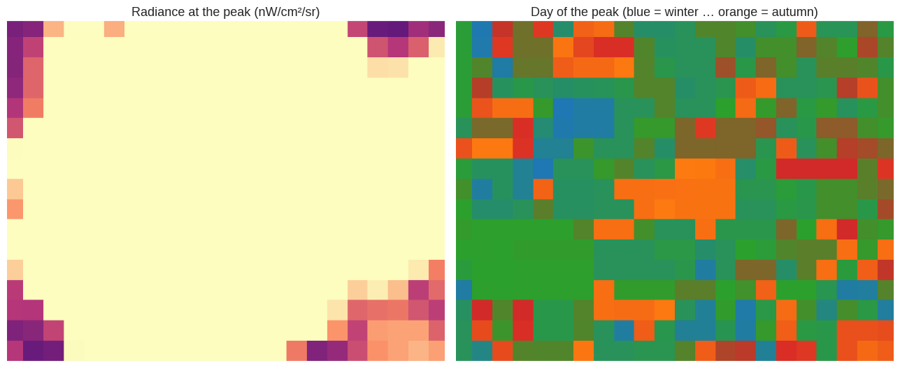
../_images/d79f142eae11679c18b637b12d812da2802a934af4f9c36ef9d6f722aeaa2ef6.png

The radiance map is the expected one: the bridges, the main avenues and the industrial estates. The timing map is not — it has structure. Blocks of pixels share a peak night, which is what a real event looks like: a fairground lights up as a unit, a street does not light up pixel by pixel.

6. Monthly instead of daily#

The same question at the resolution of the paper: which month does each pixel peak in? Cheaper, less noisy, and the unit most studies use. The only change is periods=12 and the monthly collection.

monthly = NdviSeasonality(roi=SEVILLE, sat='VIIRS', index='avg_rad', key='mean',
                          periods=12, start_year=2014, end_year=2023)

peak_month = monthly.get_peak_period(mask_below=5, return_ties=True)

hist = peak_month.select('peak_period').reduceRegion(
    ee.Reducer.frequencyHistogram(), SEVILLE, 500, maxPixels=1e9
).getInfo()['peak_period']
months = pd.Series({monthly.period_names[int(float(k)) - 1]: round(v)
                    for k, v in hist.items()}, name='pixels')
months.reindex(monthly.period_names).fillna(0).astype(int).to_frame().T

There we go again...
VIIRS DNB monthly nighttime lights (2014-present, ~500m resolution)

Year 2014: 12/12 periods with data using avg_rad index

Year 2015: 12/12 periods with data using avg_rad index

Year 2016: 12/12 periods with data using avg_rad index

Year 2017: 12/12 periods with data using avg_rad index

Year 2018: 12/12 periods with data using avg_rad index

Year 2019: 12/12 periods with data using avg_rad index

Year 2020: 12/12 periods with data using avg_rad index

Year 2021: 12/12 periods with data using avg_rad index

Year 2022: 12/12 periods with data using avg_rad index

Year 2023: 12/12 periods with data using avg_rad index

	january	february	march	april	may	june	july	august	september	october	november	december
pixels	10	20	65	48	45	69	14	14	7	1	5	13

At monthly resolution and averaged over ten years, the peak spreads across March, June, April and May — spring and early summer — with October almost empty.

This is the shape the paper works with, and it is worth understanding why it is not “December, because of Christmas lights”. The DNB sees the total radiance leaving the surface, which depends on how clear the sky was, how much of the light is scattered back, and how long the night is. In a Mediterranean spring the air is dry and clean and the city is bright; in an Atlantic December it is humid and often overcast. A festivity has to be big enough to beat that seasonal background — and the Feria, concentrated in one neighbourhood for one week, is exactly the kind of signal that survives it locally and disappears when the whole city is averaged.

7. Forty years of coast#

The second half of the notebook changes the question from when to how much, and the area from a city to the Andalusian coast — the strip that went from fishing villages to a continuous line of towns, greenhouses and resorts.

No single sensor covers it. DMSP-OLS runs 1992-2013 and VIIRS from 2014, so the series has a seam in the middle, and the two sides are not the same measurement:

DMSP is a 6-bit digital number (0-63) that saturates over city centres, with no calibration between satellites or years.
VIIRS is a calibrated radiance in nW/cm²/sr with no saturation in practice.

Converting one into the other is a research problem of its own. What can be done honestly is to read each side on its own terms and compare patterns, not values.

COAST = ee.Geometry.Rectangle([-7.5, 36.0, -1.6, 37.3])

dmsp = NdviSeasonality(roi=COAST, sat='DMSP', index='stable_lights', key='mean',
                       periods=1, start_year=1992, end_year=2013)
dmsp_years = dmsp.get_year_composite()

viirs = NdviSeasonality(roi=COAST, sat='VIIRS', index='avg_rad', key='median',
                        periods=1, start_year=2014, end_year=2025)
viirs_years = viirs.get_year_composite()

print('DMSP years: ', dmsp_years.size().getInfo())
print('VIIRS years:', viirs_years.size().getInfo())

There we go again...
DMSP-OLS annual nighttime lights (1992-2013, ~1km resolution)

Year 1992: 1/1 periods with data using stable_lights index

Year 1993: 1/1 periods with data using stable_lights index

Year 1994: 1/1 periods with data using stable_lights index

Year 1995: 1/1 periods with data using stable_lights index

Year 1996: 1/1 periods with data using stable_lights index
Year 1997: 1/1 periods with data using stable_lights index

Year 1998: 1/1 periods with data using stable_lights index

Year 1999: 1/1 periods with data using stable_lights index

Year 2000: 1/1 periods with data using stable_lights index

Year 2001: 1/1 periods with data using stable_lights index

Year 2002: 1/1 periods with data using stable_lights index

Year 2003: 1/1 periods with data using stable_lights index

Year 2004: 1/1 periods with data using stable_lights index
Year 2005: 1/1 periods with data using stable_lights index

Year 2006: 1/1 periods with data using stable_lights index

Year 2007: 1/1 periods with data using stable_lights index

Year 2008: 1/1 periods with data using stable_lights index

Year 2009: 1/1 periods with data using stable_lights index

Year 2010: 1/1 periods with data using stable_lights index

Year 2011: 1/1 periods with data using stable_lights index

Year 2012: 1/1 periods with data using stable_lights index

Year 2013: 1/1 periods with data using stable_lights index
There we go again...
VIIRS DNB monthly nighttime lights (2014-present, ~500m resolution)
  Note: VIIRS is monthly, so periods=1 averages several months per period; periods=12 keeps each month

Year 2014: 1/1 periods with data using avg_rad index

Year 2015: 1/1 periods with data using avg_rad index

Year 2016: 1/1 periods with data using avg_rad index

Year 2017: 1/1 periods with data using avg_rad index

Year 2018: 1/1 periods with data using avg_rad index

Year 2019: 1/1 periods with data using avg_rad index

Year 2020: 1/1 periods with data using avg_rad index

Year 2021: 1/1 periods with data using avg_rad index

Year 2022: 1/1 periods with data using avg_rad index

Year 2023: 1/1 periods with data using avg_rad index

Year 2024: 1/1 periods with data using avg_rad index

Year 2025: 1/1 periods with data using avg_rad index

DMSP years:  22

VIIRS years: 12

periods=1 makes each year a single composite, which is the only thing DMSP supports — it has one image per year, so there is nothing to resolve within it. The years then are the series.

def lit_area(collection, threshold, years, scale=1000):
    """Square kilometres above a brightness threshold, year by year."""
    rows = []
    images = collection.toList(collection.size())
    for i, year in enumerate(years):
        image = ee.Image(images.get(i)).select(0)
        area = (image.gte(threshold).selfMask()
                .multiply(ee.Image.pixelArea()).divide(1e6)
                .reduceRegion(ee.Reducer.sum(), COAST, scale, maxPixels=1e9)
                .getInfo())
        rows.append({'year': year, 'km2': list(area.values())[0] or 0})
    return pd.DataFrame(rows).set_index('year')['km2']

# Thresholds are not equivalent: 20 DN of DMSP and 5 nW/cm2/sr of VIIRS are
# both "clearly a town", but they are different quantities
dmsp_lit = lit_area(dmsp_years, 20, range(1992, 2014))
viirs_lit = lit_area(viirs_years, 5, range(2014, 2026), scale=500)

summary = pd.DataFrame({
    'first year': [dmsp_lit.index[0], viirs_lit.index[0]],
    'first km²': [dmsp_lit.iloc[0], viirs_lit.iloc[0]],
    'last year': [dmsp_lit.index[-1], viirs_lit.index[-1]],
    'last km²': [dmsp_lit.iloc[-1], viirs_lit.iloc[-1]],
}, index=['DMSP-OLS', 'VIIRS'])
summary['growth'] = summary['last km²'] / summary['first km²'] - 1
print(summary.round(1).to_string())

          first year  first km²  last year  last km²  growth
DMSP-OLS        1992     4207.9       2013    7887.9     0.9
VIIRS           2014     2908.6       2025    3182.6     0.1

fig, ax = plt.subplots(figsize=(10, 4.5))
ax.plot(dmsp_lit.index, dmsp_lit.values, 'o-', color='#8c564b', label='DMSP-OLS (DN ≥ 20)')
ax.plot(viirs_lit.index, viirs_lit.values, 'o-', color='#1f77b4',
        label='VIIRS (≥ 5 nW/cm²/sr)')
ax.axvspan(2013, 2014, color='0.9')
ax.text(2013.5, ax.get_ylim()[1] * 0.95, 'sensor change', ha='center', fontsize=8,
        color='0.4')
ax.set_ylabel('Lit area (km²)')
ax.set_title('Lit area of the Andalusian coast, two incomparable rulers')
ax.legend(frameon=False)
for side in ('top', 'right'):
    ax.spines[side].set_visible(False)
plt.tight_layout()

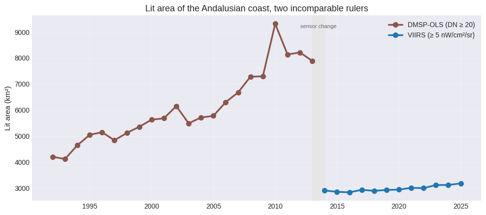
../_images/2f704553b3eaf73eb4d036bc585a6b603ed0b83311bc2886dd88e67a4bbeeda0.png

Two ascending lines that must not be joined into one. The lit area runs from 4,208 km² in 1992 to 7,888 km² in 2013 on DMSP (+90%), and from 2,909 km² in 2014 to 3,183 km² in 2025 on VIIRS (+9%). The drop of five thousand square kilometres at the seam is the change of instrument, not a blackout: DN ≥ 20 and ≥ 5 nW/cm²/sr are two different definitions of “lit”, and DMSP’s coarse optics smear a town’s light over neighbouring kilometres, which inflates any area measured from it.

Even the +90% is not all construction. DMSP was flown by a succession of satellites whose digital numbers were never calibrated against each other, so part of that slope is the instrument drifting. Published DMSP time series apply an intercalibration — a per-year regression against a reference scene — before reading any trend, and this notebook deliberately does not: the point here is the shape of the two records and where they can and cannot be joined.

What survives all those caveats is the direction, which both halves agree on and which the maps below show directly: the coast filled in, fastest during the building boom of the DMSP years.

lights_vis_dmsp = {'min': 0, 'max': 63, 'palette': ['000000', 'ffd27f', 'ffffff']}
lights_vis_viirs = {'min': 0, 'max': 40, 'palette': ['000000', 'ffd27f', 'ffffff']}

fig, axes = plt.subplots(2, 2, figsize=(13, 7))
pairs = [(ee.Image(dmsp_years.toList(30).get(0)), lights_vis_dmsp, 'DMSP 1992'),
         (ee.Image(dmsp_years.toList(30).get(21)), lights_vis_dmsp, 'DMSP 2013'),
         (ee.Image(viirs_years.toList(30).get(0)), lights_vis_viirs, 'VIIRS 2014'),
         (ee.Image(viirs_years.toList(30).get(11)), lights_vis_viirs, 'VIIRS 2025')]
for ax, (image, vis, title) in zip(axes.ravel(), pairs):
    ax.imshow(thumbnail(image.select(0), vis, COAST, dimensions=700))
    ax.set_title(title)
    ax.axis('off')
plt.tight_layout()

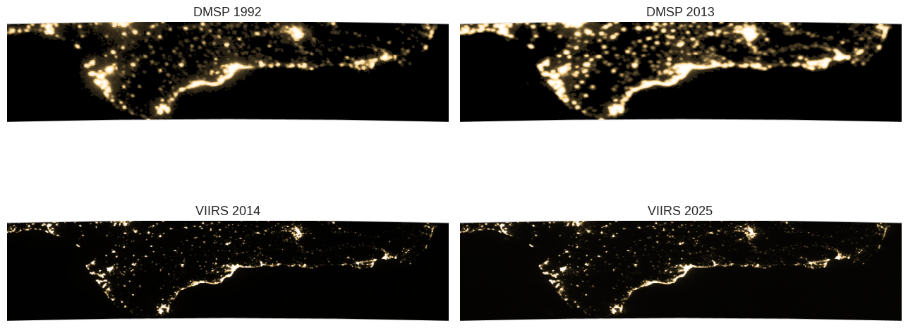
../_images/ef1ce86cd9378252f76947793b8744c0768d98bdf44589cd29ebedc56728f506.png

The four maps are the same coast through two instruments. Between 1992 and 2013 the change is unmistakable: the Costa del Sol becomes a continuous ribbon of light from Málaga to Estepona, and the greenhouse sea around El Ejido appears out of the dark.

Note what DMSP does to a city centre: it saturates. Málaga and Seville are flat white blobs in 1992 and flat white blobs in 2013, so the growth that the map shows is growth at the edges, where the sensor still has range. VIIRS, with no saturation, resolves the structure inside the cities — which is another reason the two halves of the record cannot be compared value by value.

8. What to take away#

A local peak is an event; a shared peak is the atmosphere. The Feria week holds the maximum of a third of the fairground’s pixels and of none of the historic centre’s. A single night in March holds the maximum of a quarter of the fairground and a third of the centre. The first is a fair; the second is a clear night. Nothing but the spatial pattern separates them, which is why get_peak_period() returns a map and not a date.

Ask the question where the answer can be local. Averaged over the whole city, the Feria is invisible: the monthly map peaks in spring because springs are clear, not because anything happened. The signal exists at the scale of the event.

Not every celebration is a light. Holy Week, which fills the same city for a week, is indistinguishable from chance. Processions are lit at street level, under cover and often by candle: the sensor is looking straight down at rooftops.

Ties and coverage are part of the answer. return_ties=True and a count of valid observations per period cost one line each and tell you whether the map is reporting a measurement or rounding noise.

Two records are not one record. DMSP and VIIRS both measure nighttime light, and the seam between them cannot be crossed by rescaling a threshold. Read each on its own terms, compare patterns rather than values, and say so in the caption.